Info

This article grew out of my Beamer slide deck, From Words to Attention: The Road to the Transformer. It is not meant to be a complete Transformer tutorial. It is closer to a reconstruction of the path that made Transformers click for me: an NLP architecture first, and then a more general way to model dependencies between tokens.

The problem before the Transformer

It is tempting to explain the Transformer by starting with the equation:

$$\mathrm{Attention}(Q,K,V)=\mathrm{softmax}\left(\frac{QK^\top}{\sqrt{d_k}}\right)V.$$

That equation matters, but for me it starts too late. The more useful question is simpler:

How can a machine represent words in a way that preserves meaning, context, and relationships?

The Transformer is one answer to that question, but it only makes sense after seeing the earlier answers fail in very specific ways. One-hot vectors solved identity but not similarity. N-gram models gave local context but not much abstraction. Word embeddings gave geometry but not dynamic meaning. Recurrent networks gave state, but long-range information still had to survive a long serial path. Attention changed the shape of the information flow: instead of squeezing everything through one narrow temporal corridor, each position could ask the rest of the sequence what mattered right now.

That is the storyline I want to preserve from the slides.

Start with discrete symbols

The earliest representation is brutally simple: each word is an index in a vocabulary. A one-hot vector has one active coordinate. Everything else is zero.

For a vocabulary $\mathcal{V}$, a word $w_i$ can be represented as:

$$\mathbf{x}_i = [0,\dots,0,1,0,\dots,0] \in \mathbb{R}^{|\mathcal{V}|}.$$

This representation is clean for lookup. It tells the model exactly which symbol occurred. But it says nothing about what the symbol means. "cat" and "dog" are as far apart as "cat" and "parliament" if we use raw one-hot distance. Every pair of distinct words is equally unrelated.

N-gram models add a little bit of sequence awareness. Instead of asking only "what is this word?", they ask "what word usually follows the previous $n-1$ words?" A trigram model estimates:

$$P(w_t \mid w_{t-2}, w_{t-1}).$$

This works surprisingly well for small local patterns, but the boundary is hard: the context window is fixed, discrete, and sparse. If a phrase was rarely seen, the model has little room to generalize. If the relevant dependency is outside the window, the model cannot see it.

I remember this part as a useful negative result:

Symbolic representations preserve identity, but they do not preserve semantic distance.

Word vectors give meaning a geometry

The next step is to replace symbolic identity with continuous representation. Bengio's neural language model and the later Word2Vec family made this shift feel concrete: a word is no longer just a vocabulary index. It becomes a vector learned from context.

Instead of manually defining similarity, we learn an embedding matrix:

$$E \in \mathbb{R}^{|\mathcal{V}| \times d}.$$

The row $E_i$ becomes the vector for word $w_i$. Words used in similar contexts end up near each other. Suddenly there is a geometry of meaning. Cosine similarity becomes useful. Analogies become possible. The model can share statistical strength between words nobody explicitly connected by hand.

This was a real conceptual leap. It changed "language as dictionary lookup" into "language as geometry."

But static embeddings also hide a problem. A word type receives one vector. The word "bank" has one representation whether it appears in "river bank" or "investment bank." The context may be nearby in the sentence, but the embedding itself is fixed before the sentence is read.

So this step solves one problem and leaves another:

Continuous vectors solve semantic similarity, but a static vector cannot fully represent context-dependent meaning.

Sequences need memory, but the road is long

Recurrent neural networks address the context problem by processing tokens one at a time and carrying a hidden state:

$$\mathbf{h}_t = f(\mathbf{x}_t, \mathbf{h}_{t-1}).$$

Now the representation at time $t$ depends on what came before it. That is already a big improvement. The model is no longer looking at words in isolation. It is building a running summary as it reads.

LSTMs improve this further by adding gated memory. Instead of overwriting state blindly, they learn when to write, when to forget, and when to expose information. The memory becomes less like a scratchpad and more like something the model can manage.

But the structure is still sequential. To connect token 1 and token 80, information has to travel through many intermediate states. During training, gradients also travel through that chain. This leads to two practical issues:

• Long-distance dependencies are hard to preserve.
• Computation is hard to parallelize across time.

The hidden state is useful, but it is also a narrow corridor. It carries context, but every token has to pass through the same temporal path.

That tension is what I associate with the recurrent era:

Recurrence makes meaning dynamic, but it makes information flow sequential and fragile.

Seq2Seq bottleneck

Sequence-to-sequence models made the problem hard to ignore. In machine translation, an encoder reads the source sentence and compresses it into a context vector. A decoder then generates the target sentence from that vector.

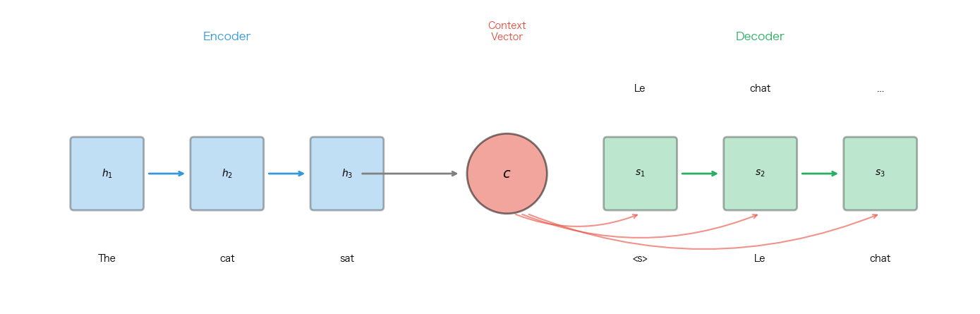
A fixed-context encoder-decoder model asks one vector to summarize the whole source sequence.

The abstraction is neat:

$$\mathbf{c} = \mathbf{h}_T, \qquad P(y_t \mid y_{<t}, x_{1:T}) = g(y_{t-1}, \mathbf{s}_{t-1}, \mathbf{c}).$$

The encoder gives the decoder one final summary $\mathbf{c}$. The decoder uses that same vector at every generation step.

The weakness is also obvious. A short sentence may fit into a single vector. A long sentence with gender agreement, subordinate clauses, pronoun references, and word reordering probably should not.

Imagine translating:

The book is on the table because it is too slippery.

Depending on the target language, "it" may need to agree with "book" or "table." The decoder should be able to look back at the specific source token that matters at the moment of generation. A single fixed vector asks the model to remember everything before it knows what will be needed.

The issue is not that the encoder learned nothing. The interface is too narrow:

The bottleneck is not that the encoder has no information. The bottleneck is that the decoder cannot selectively retrieve it.

Attention as dynamic retrieval

Attention changes the interface between encoder and decoder. Instead of giving the decoder only the final state, we keep all encoder states:

$$\mathbf{h}_1,\mathbf{h}_2,\dots,\mathbf{h}_T.$$

At decoding step $t$, the decoder computes alignment scores:

$$e_{t,i} = a(\mathbf{s}_{t-1}, \mathbf{h}_i),$$

then normalizes them:

$$\alpha_{t,i} = \frac{\exp(e_{t,i})}{\sum_j \exp(e_{t,j})},$$

and builds a step-specific context:

$$\mathbf{c}_t = \sum_i \alpha_{t,i}\mathbf{h}_i.$$

Now each output token gets a different context vector. The decoder no longer asks the encoder to compress everything into one summary. It asks a more specific question:

For the thing I am generating right now, which source positions matter?

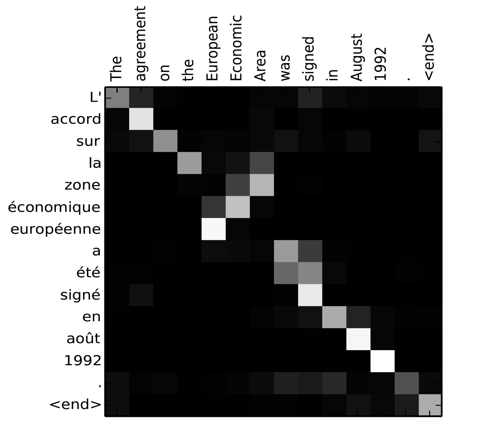
Soft attention turns translation into learned alignment. The important source positions can change at each output step.

This was the turning point for me. Attention is often introduced as a matrix trick, but the idea is closer to retrieval. A query asks for something. Keys decide what matches. Values provide the content that gets mixed.

Put differently:

Attention replaces one global memory with many step-specific reads from memory.

Self-attention removes the recurrent chain

The next move is simple, almost annoyingly so. If attention helps the decoder read from the source sequence, why not let tokens in the same sequence read from one another?

That is self-attention. Each token produces a query, key, and value:

$$Q=XW_Q,\qquad K=XW_K,\qquad V=XW_V.$$

The sequence updates itself by comparing all positions against all other positions:

$$\mathrm{softmax}\left(\frac{QK^\top}{\sqrt{d_k}}\right)V.$$

The important difference is structural. In an RNN, token 80 receives information from token 1 through a chain of hidden states. In self-attention, token 80 can attend to token 1 directly in one layer.

This is why I think of self-attention as a soft graph over tokens. The graph is not fixed in advance. Its edge weights are computed from the current representations. A pronoun can look at its antecedent. A verb can look at its subject. An image patch can look at another patch. The model is not handed a dependency graph before computation; it grows one while computing.

This is the part I keep coming back to:

Self-attention makes dependency modelling direct, parallel, and content-dependent.

Transformer recipe

The Transformer wraps self-attention in a full recipe:

• Token embeddings turn discrete input into vectors.
• Positional encodings inject order because self-attention alone is permutation-invariant.
• Multi-head attention lets the model attend through several learned relation spaces at once.
• Residual connections and layer normalization make deep composition trainable.
• Feed-forward layers transform each contextualized token locally.
• Masking controls which positions are visible during generation.
• Encoder-decoder attention lets the decoder read from encoded source states.

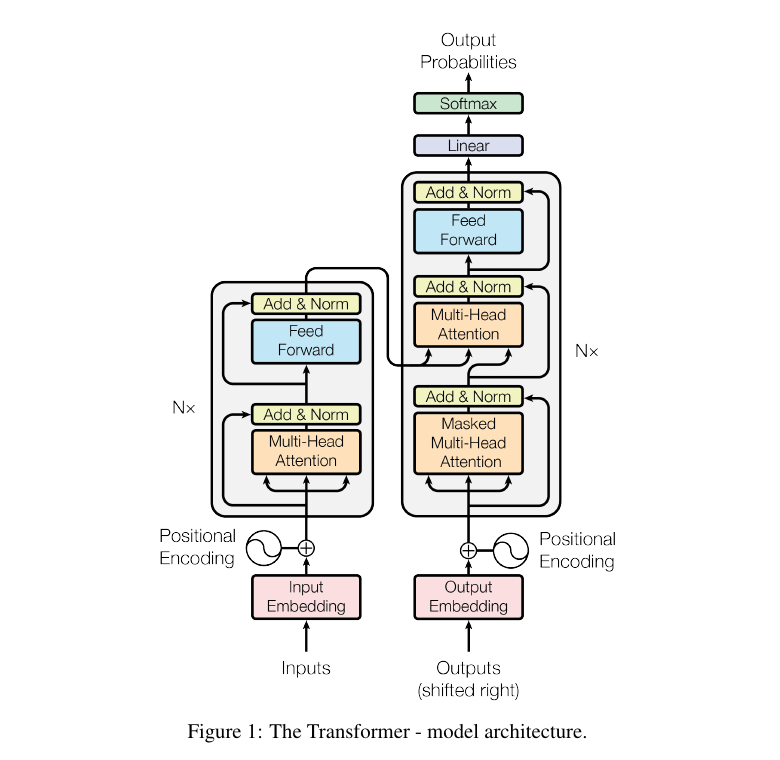
The original Transformer combines self-attention, cross-attention, position information, residual paths, and local feed-forward transformations.

Multi-head attention is worth pausing on. A single attention head may focus on one kind of relation. Several heads can distribute the work: syntax, agreement, nearby context, long-range reference, delimiter structure, or task-specific alignment. We should not over-interpret individual heads too literally, but the architectural idea is clear: do not force every relation through one similarity function.

At this point the Transformer stops being only an NLP trick. It becomes a general way to update a set or sequence of tokens by learned pairwise interaction.

At this point my mental model of the Transformer becomes:

Once everything is a token, attention becomes a general dependency engine.

What happens beyond text

The final section of the slides asks why Transformers spread so far beyond machine translation. My answer is that the core operation is not tied very tightly to language.

Text is already a sequence of tokens. Images can be divided into patches. Audio can be divided into frames. Video can be represented by space-time patches. A 3D scene can be represented with views, points, or latent tokens. Once the input becomes tokens, the same question reappears:

Which tokens should interact, and how strongly?

ViT showed that image patches can be processed by a Transformer encoder. CLIP showed that text and images can be aligned in one shared embedding space. Diffusion systems use cross-attention so prompts can condition image generation. Multimodal LLMs project visual tokens into language-model space. Video and 3D systems extend the same pattern across time and view geometry.

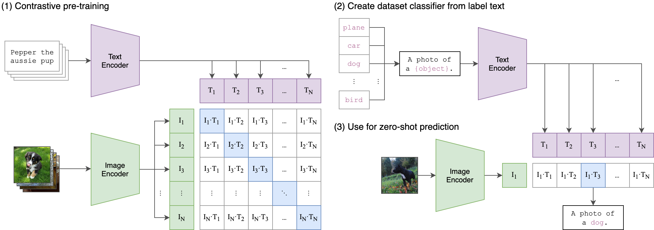
CLIP turns image-text matching into geometry: matched pairs are pulled together, non-matching pairs are pushed apart.

The point is not that every problem becomes language. The point is that many problems can be represented as interacting tokens.

That is the summary I still find useful:

The Transformer became powerful because it separated the general operation from the modality-specific front end. Tokenization changes. Conditioning changes. The attention primitive remains.

What I took away

The story from words to attention is not a straight line of bigger models. It is a sequence of pressure points:

Stage	What It Solved	What Still Hurt
One-hot	Exact identity	No semantic distance
N-gram	Local context	Sparse, fixed window
Embeddings	Semantic geometry	Static meaning
RNN/LSTM	Dynamic sequence state	Long chains, weak parallelism
Seq2seq	Variable input to variable output	Fixed context bottleneck
Attention	Dynamic retrieval	Still attached to recurrence
Self-attention	Direct token interaction	Needs position and architecture around it
Transformer	Scalable dependency modelling	Cost grows with sequence length

That is why I find the Transformer easier to understand historically than algebraically. The algebra is compact. The motivation is cumulative.

The model is not magical because it has a softmax over dot products. It is powerful because it changes the default communication pattern inside a model. Instead of passing information through a single recurrent thread, it lets every token ask the rest of the context what matters.

Once I understood that, the later systems became less mysterious. ViT, CLIP, diffusion, multimodal LLMs, and video models are not unrelated inventions. They are variations on the same design principle:

Turn the world into tokens, then learn the dependency structure among them.

References

• Yoshua Bengio et al. (2003), A Neural Probabilistic Language Model.
• Tomas Mikolov et al. (2013), Efficient Estimation of Word Representations in Vector Space.
• Kyunghyun Cho et al. (2014), Learning Phrase Representations using RNN Encoder-Decoder for Statistical Machine Translation.
• Dzmitry Bahdanau, Kyunghyun Cho, and Yoshua Bengio (2015), Neural Machine Translation by Jointly Learning to Align and Translate.
• Ashish Vaswani et al. (2017), Attention Is All You Need.
• Alexey Dosovitskiy et al. (2021), An Image is Worth 16x16 Words.
• Alec Radford et al. (2021), Learning Transferable Visual Models From Natural Language Supervision.

Contributors: Eryc123Y

Next pageAI Evolution: From Deep Learning to Large Language Models